 View on TensorFlow.org View on TensorFlow.org
|
 Run in Google Colab Run in Google Colab
|
 View on GitHub View on GitHub
|
 Download notebook Download notebook
|
 See TF Hub models See TF Hub models
|
This notebook shows you how to fine-tune CropNet models from TensorFlow Hub on a dataset from TFDS or your own crop disease detection dataset.
You will:
- Load the TFDS cassava dataset or your own data
- Enrich the data with unknown (negative) examples to get a more robust model
- Apply image augmentations to the data
- Load and fine tune a CropNet model from TF Hub
- Export a TFLite model, ready to be deployed on your app with Task Library, MLKit or TFLite directly
Imports and Dependencies
Before starting, you'll need to install some of the dependencies that will be needed like Model Maker and the latest version of TensorFlow Datasets.
sudo apt install -q libportaudio2## image_classifier library requires numpy <= 1.23.5pip install "numpy<=1.23.5"pip install --use-deprecated=legacy-resolver tflite-model-maker-nightlypip install -U tensorflow-datasets## scann library requires tensorflow < 2.9.0pip install "tensorflow<2.9.0"pip install "tensorflow-datasets~=4.8.0" # protobuf>=3.12.2pip install tensorflow-metadata~=1.10.0 # protobuf>=3.13## tensorflowjs requires packaging < 20.10pip install "packaging<20.10"
import matplotlib.pyplot as plt
import os
import seaborn as sns

import tensorflow as tf
import tensorflow_datasets as tfds

from tensorflow_examples.lite.model_maker.core.export_format import ExportFormat
from tensorflow_examples.lite.model_maker.core.task import image_preprocessing

from tflite_model_maker import image_classifier
from tflite_model_maker import ImageClassifierDataLoader
from tflite_model_maker.image_classifier import ModelSpec
2023-11-07 13:39:32.174301: W tensorflow/stream_executor/platform/default/dso_loader.cc:64] Could not load dynamic library 'libcudart.so.11.0'; dlerror: libcudart.so.11.0: cannot open shared object file: No such file or directory
/tmpfs/src/tf_docs_env/lib/python3.9/site-packages/tensorflow_addons/utils/tfa_eol_msg.py:23: UserWarning:

TensorFlow Addons (TFA) has ended development and introduction of new features.
TFA has entered a minimal maintenance and release mode until a planned end of life in May 2024.
Please modify downstream libraries to take dependencies from other repositories in our TensorFlow community (e.g. Keras, Keras-CV, and Keras-NLP).

For more information see: https://github.com/tensorflow/addons/issues/2807

  warnings.warn(
/tmpfs/src/tf_docs_env/lib/python3.9/site-packages/tensorflow_addons/utils/ensure_tf_install.py:53: UserWarning: Tensorflow Addons supports using Python ops for all Tensorflow versions above or equal to 2.12.0 and strictly below 2.15.0 (nightly versions are not supported).
 The versions of TensorFlow you are currently using is 2.8.4 and is not supported.
Some things might work, some things might not.
If you were to encounter a bug, do not file an issue.
If you want to make sure you're using a tested and supported configuration, either change the TensorFlow version or the TensorFlow Addons's version.
You can find the compatibility matrix in TensorFlow Addon's readme:
https://github.com/tensorflow/addons
  warnings.warn(
Load a TFDS dataset to fine-tune on
Lets use the publicly available Cassava Leaf Disease dataset from TFDS.
tfds_name = 'cassava'
(ds_train, ds_validation, ds_test), ds_info = tfds.load(
    name=tfds_name,
    split=['train', 'validation', 'test'],
    with_info=True,
    as_supervised=True)
TFLITE_NAME_PREFIX = tfds_name
2023-11-07 13:39:36.293577: E tensorflow/stream_executor/cuda/cuda_driver.cc:271] failed call to cuInit: CUDA_ERROR_NO_DEVICE: no CUDA-capable device is detected
Or alternatively load your own data to fine-tune on
Instead of using a TFDS dataset, you can also train on your own data. This code snippet shows how to load your own custom dataset. See this link for the supported structure of the data. An example is provided here using the publicly available Cassava Leaf Disease dataset.
# data_root_dir = tf.keras.utils.get_file(
#     'cassavaleafdata.zip',
#     'https://storage.googleapis.com/emcassavadata/cassavaleafdata.zip',
#     extract=True)
# data_root_dir = os.path.splitext(data_root_dir)[0]  # Remove the .zip extension

# builder = tfds.ImageFolder(data_root_dir)

# ds_info = builder.info
# ds_train = builder.as_dataset(split='train', as_supervised=True)
# ds_validation = builder.as_dataset(split='validation', as_supervised=True)
# ds_test = builder.as_dataset(split='test', as_supervised=True)
Visualize samples from train split
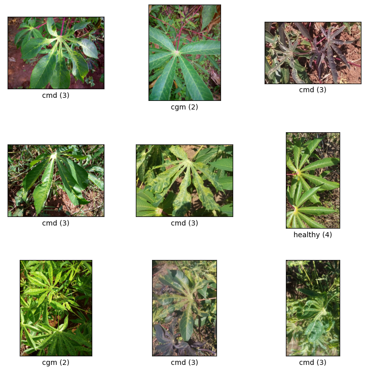
Let's take a look at some examples from the dataset including the class id and the class name for the image samples and their labels.
_ = tfds.show_examples(ds_train, ds_info)

Add images to be used as Unknown examples from TFDS datasets
Add additional unknown (negative) examples to the training dataset and assign a new unknown class label number to them. The goal is to have a model that, when used in practice (e.g. in the field), has the option of predicting "Unknown" when it sees something unexpected.
Below you can see a list of datasets that will be used to sample the additional unknown imagery. It includes 3 completely different datasets to increase diversity. One of them is a beans leaf disease dataset, so that the model has exposure to diseased plants other than cassava.
UNKNOWN_TFDS_DATASETS = [{
    'tfds_name': 'imagenet_v2/matched-frequency',
    'train_split': 'test[:80%]',
    'test_split': 'test[80%:]',
    'num_examples_ratio_to_normal': 1.0,
}, {
    'tfds_name': 'oxford_flowers102',
    'train_split': 'train',
    'test_split': 'test',
    'num_examples_ratio_to_normal': 1.0,
}, {
    'tfds_name': 'beans',
    'train_split': 'train',
    'test_split': 'test',
    'num_examples_ratio_to_normal': 1.0,
}]
The UNKNOWN datasets are also loaded from TFDS.
# Load unknown datasets.
weights = [
    spec['num_examples_ratio_to_normal'] for spec in UNKNOWN_TFDS_DATASETS
]
num_unknown_train_examples = sum(
    int(w * ds_train.cardinality().numpy()) for w in weights)
ds_unknown_train = tf.data.Dataset.sample_from_datasets([
    tfds.load(
        name=spec['tfds_name'], split=spec['train_split'],
        as_supervised=True).repeat(-1) for spec in UNKNOWN_TFDS_DATASETS
], weights).take(num_unknown_train_examples)
ds_unknown_train = ds_unknown_train.apply(
    tf.data.experimental.assert_cardinality(num_unknown_train_examples))
ds_unknown_tests = [
    tfds.load(
        name=spec['tfds_name'], split=spec['test_split'], as_supervised=True)
    for spec in UNKNOWN_TFDS_DATASETS
]
ds_unknown_test = ds_unknown_tests[0]
for ds in ds_unknown_tests[1:]:
  ds_unknown_test = ds_unknown_test.concatenate(ds)

# All examples from the unknown datasets will get a new class label number.
num_normal_classes = len(ds_info.features['label'].names)
unknown_label_value = tf.convert_to_tensor(num_normal_classes, tf.int64)
ds_unknown_train = ds_unknown_train.map(lambda image, _:
                                        (image, unknown_label_value))
ds_unknown_test = ds_unknown_test.map(lambda image, _:
                                      (image, unknown_label_value))

# Merge the normal train dataset with the unknown train dataset.
weights = [
    ds_train.cardinality().numpy(),
    ds_unknown_train.cardinality().numpy()
]
ds_train_with_unknown = tf.data.Dataset.sample_from_datasets(
    [ds_train, ds_unknown_train], [float(w) for w in weights])
ds_train_with_unknown = ds_train_with_unknown.apply(
    tf.data.experimental.assert_cardinality(sum(weights)))

print((f"Added {ds_unknown_train.cardinality().numpy()} negative examples."
       f"Training dataset has now {ds_train_with_unknown.cardinality().numpy()}"
       ' examples in total.'))
Added 16968 negative examples.Training dataset has now 22624 examples in total.
Apply augmentations
For all the images, to make them more diverse, you'll apply some augmentation, like changes in:
- Brightness
- Contrast
- Saturation
- Hue
- Crop
These types of augmentations help make the model more robust to variations in image inputs.
def random_crop_and_random_augmentations_fn(image):
  # preprocess_for_train does random crop and resize internally.
  image = image_preprocessing.preprocess_for_train(image)
  image = tf.image.random_brightness(image, 0.2)
  image = tf.image.random_contrast(image, 0.5, 2.0)
  image = tf.image.random_saturation(image, 0.75, 1.25)
  image = tf.image.random_hue(image, 0.1)
  return image


def random_crop_fn(image):
  # preprocess_for_train does random crop and resize internally.
  image = image_preprocessing.preprocess_for_train(image)
  return image


def resize_and_center_crop_fn(image):
  image = tf.image.resize(image, (256, 256))
  image = image[16:240, 16:240]
  return image


no_augment_fn = lambda image: image

train_augment_fn = lambda image, label: (
    random_crop_and_random_augmentations_fn(image), label)
eval_augment_fn = lambda image, label: (resize_and_center_crop_fn(image), label)
To apply the augmentation, it uses the map method from the Dataset class.
ds_train_with_unknown = ds_train_with_unknown.map(train_augment_fn)
ds_validation = ds_validation.map(eval_augment_fn)
ds_test = ds_test.map(eval_augment_fn)
ds_unknown_test = ds_unknown_test.map(eval_augment_fn)
INFO:tensorflow:Use default resize_bicubic.
INFO:tensorflow:Use default resize_bicubic.
INFO:tensorflow:Use customized resize method bilinear
INFO:tensorflow:Use customized resize method bilinear
Wrap the data into Model Maker friendly format
To use these dataset with Model Maker, they need to be in a ImageClassifierDataLoader class.
label_names = ds_info.features['label'].names + ['UNKNOWN']

train_data = ImageClassifierDataLoader(ds_train_with_unknown,
                                       ds_train_with_unknown.cardinality(),
                                       label_names)
validation_data = ImageClassifierDataLoader(ds_validation,
                                            ds_validation.cardinality(),
                                            label_names)
test_data = ImageClassifierDataLoader(ds_test, ds_test.cardinality(),
                                      label_names)
unknown_test_data = ImageClassifierDataLoader(ds_unknown_test,
                                              ds_unknown_test.cardinality(),
                                              label_names)
Run training
TensorFlow Hub has multiple models available for Transfer Learning.
Here you can choose one and you can also keep experimenting with other ones to try to get better results.
If you want even more models to try, you can add them from this collection.
Choose a base model
model_name = 'mobilenet_v3_large_100_224'

map_model_name = {
    'cropnet_cassava':
        'https://tfhub.dev/google/cropnet/feature_vector/cassava_disease_V1/1',
    'cropnet_concat':
        'https://tfhub.dev/google/cropnet/feature_vector/concat/1',
    'cropnet_imagenet':
        'https://tfhub.dev/google/cropnet/feature_vector/imagenet/1',
    'mobilenet_v3_large_100_224':
        'https://tfhub.dev/google/imagenet/mobilenet_v3_large_100_224/feature_vector/5',
}

model_handle = map_model_name[model_name]
To fine tune the model, you will use Model Maker. This makes the overall solution easier since after the training of the model, it'll also convert it to TFLite.
Model Maker makes this conversion be the best one possible and with all the necessary information to easily deploy the model on-device later.
The model spec is how you tell Model Maker which base model you'd like to use.
image_model_spec = ModelSpec(uri=model_handle)
One important detail here is setting train_whole_model which will make the base model fine tuned during training. This makes the process slower but the final model has a higher accuracy. Setting shuffle will make sure the model sees the data in a random shuffled order which is a best practice for model learning.
model = image_classifier.create(
    train_data,
    model_spec=image_model_spec,
    batch_size=128,
    learning_rate=0.03,
    epochs=5,
    shuffle=True,
    train_whole_model=True,
    validation_data=validation_data)
INFO:tensorflow:Retraining the models...
INFO:tensorflow:Retraining the models...
Model: "sequential"
_________________________________________________________________
 Layer (type)                Output Shape              Param #
=================================================================
 hub_keras_layer_v1v2 (HubKe  (None, 1280)             4226432
 rasLayerV1V2)

 dropout (Dropout)           (None, 1280)              0

 dense (Dense)               (None, 6)                 7686

=================================================================
Total params: 4,234,118
Trainable params: 4,209,718
Non-trainable params: 24,400
_________________________________________________________________
None
Epoch 1/5
176/176 [==============================] - 485s 3s/step - loss: 0.8830 - accuracy: 0.9190 - val_loss: 1.1238 - val_accuracy: 0.8068
Epoch 2/5
176/176 [==============================] - 463s 3s/step - loss: 0.7892 - accuracy: 0.9545 - val_loss: 1.0590 - val_accuracy: 0.8290
Epoch 3/5
176/176 [==============================] - 464s 3s/step - loss: 0.7744 - accuracy: 0.9577 - val_loss: 1.0222 - val_accuracy: 0.8438
Epoch 4/5
176/176 [==============================] - 463s 3s/step - loss: 0.7617 - accuracy: 0.9633 - val_loss: 1.0435 - val_accuracy: 0.8407
Epoch 5/5
176/176 [==============================] - 461s 3s/step - loss: 0.7571 - accuracy: 0.9653 - val_loss: 0.9859 - val_accuracy: 0.8655
Evaluate model on test split
model.evaluate(test_data)
59/59 [==============================] - 7s 101ms/step - loss: 0.9668 - accuracy: 0.8637
[0.9668245911598206, 0.863660454750061]
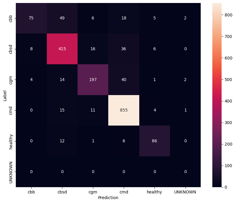
To have an even better understanding of the fine tuned model, it's good to analyse the confusion matrix. This will show how often one class is predicted as another.
def predict_class_label_number(dataset):
  """Runs inference and returns predictions as class label numbers."""
  rev_label_names = {l: i for i, l in enumerate(label_names)}
  return [
      rev_label_names[o[0][0]]
      for o in model.predict_top_k(dataset, batch_size=128)
  ]

def show_confusion_matrix(cm, labels):
  plt.figure(figsize=(10, 8))
  sns.heatmap(cm, xticklabels=labels, yticklabels=labels,
              annot=True, fmt='g')
  plt.xlabel('Prediction')
  plt.ylabel('Label')
  plt.show()
confusion_mtx = tf.math.confusion_matrix(
    list(ds_test.map(lambda x, y: y)),
    predict_class_label_number(test_data),
    num_classes=len(label_names))

show_confusion_matrix(confusion_mtx, label_names)

Evaluate model on unknown test data
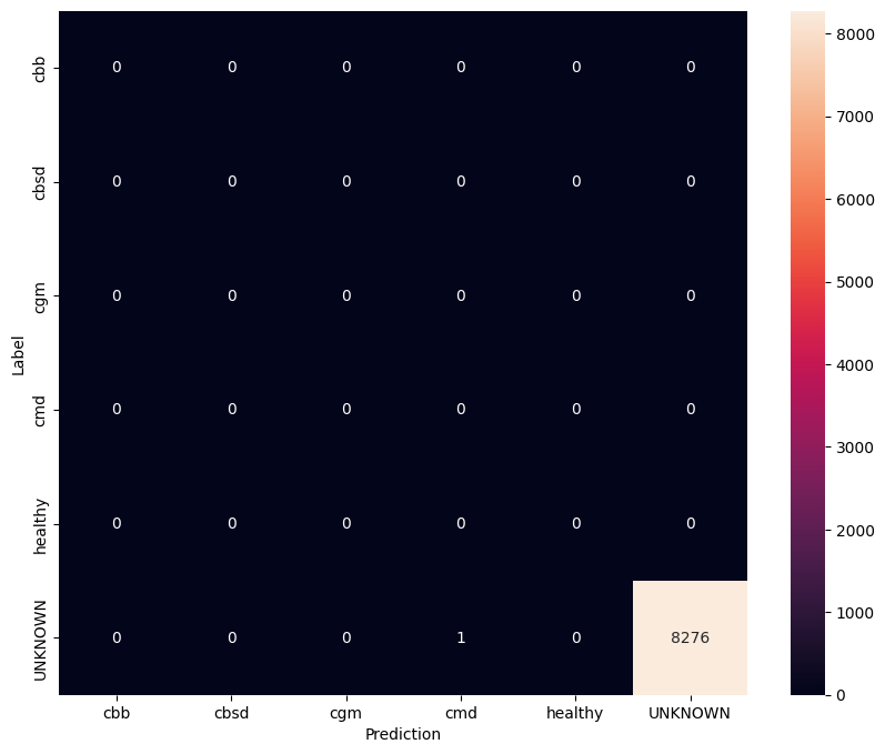
In this evaluation we expect the model to have accuracy of almost 1. All images the model is tested on are not related to the normal dataset and hence we expect the model to predict the "Unknown" class label.
model.evaluate(unknown_test_data)
259/259 [==============================] - 30s 111ms/step - loss: 0.6760 - accuracy: 0.9999
[0.6760221719741821, 0.9998791813850403]
Print the confusion matrix.
unknown_confusion_mtx = tf.math.confusion_matrix(
    list(ds_unknown_test.map(lambda x, y: y)),
    predict_class_label_number(unknown_test_data),
    num_classes=len(label_names))

show_confusion_matrix(unknown_confusion_mtx, label_names)

Export the model as TFLite and SavedModel
Now we can export the trained models in TFLite and SavedModel formats for deploying on-device and using for inference in TensorFlow.
tflite_filename = f'{TFLITE_NAME_PREFIX}_model_{model_name}.tflite'
model.export(export_dir='.', tflite_filename=tflite_filename)
2023-11-07 14:20:20.089818: W tensorflow/python/util/util.cc:368] Sets are not currently considered sequences, but this may change in the future, so consider avoiding using them.
INFO:tensorflow:Assets written to: /tmpfs/tmp/tmp99qci6gx/assets
INFO:tensorflow:Assets written to: /tmpfs/tmp/tmp99qci6gx/assets
/tmpfs/src/tf_docs_env/lib/python3.9/site-packages/tensorflow/lite/python/convert.py:746: UserWarning: Statistics for quantized inputs were expected, but not specified; continuing anyway.
  warnings.warn("Statistics for quantized inputs were expected, but not "
2023-11-07 14:20:30.245779: W tensorflow/compiler/mlir/lite/python/tf_tfl_flatbuffer_helpers.cc:357] Ignored output_format.
2023-11-07 14:20:30.245840: W tensorflow/compiler/mlir/lite/python/tf_tfl_flatbuffer_helpers.cc:360] Ignored drop_control_dependency.
fully_quantize: 0, inference_type: 6, input_inference_type: 3, output_inference_type: 3
INFO:tensorflow:Label file is inside the TFLite model with metadata.
INFO:tensorflow:Label file is inside the TFLite model with metadata.
INFO:tensorflow:Saving labels in /tmpfs/tmp/tmp8co343h3/labels.txt
INFO:tensorflow:Saving labels in /tmpfs/tmp/tmp8co343h3/labels.txt
INFO:tensorflow:TensorFlow Lite model exported successfully: ./cassava_model_mobilenet_v3_large_100_224.tflite
INFO:tensorflow:TensorFlow Lite model exported successfully: ./cassava_model_mobilenet_v3_large_100_224.tflite
# Export saved model version.
model.export(export_dir='.', export_format=ExportFormat.SAVED_MODEL)
INFO:tensorflow:Assets written to: ./saved_model/assets
INFO:tensorflow:Assets written to: ./saved_model/assets
Next steps
The model that you've just trained can be used on mobile devices and even deployed in the field!
To download the model, click the folder icon for the Files menu on the left side of the colab, and choose the download option.
The same technique used here could be applied to other plant diseases tasks that might be more suitable for your use case or any other type of image classification task. If you want to follow up and deploy on an Android app, you can continue on this Android quickstart guide.
