Overview
The main feature of TensorBoard is its interactive GUI. However, users sometimes want to programmatically read the data logs stored in TensorBoard, for purposes such as performing post-hoc analyses and creating custom visualizations of the log data.
TensorBoard 2.3 supports this use case with tensorboard.data.experimental.ExperimentFromDev(). It allows programmatic access to TensorBoard's scalar logs. This page demonstrates the basic usage of this new API.
Setup
In order to use the programmatic API, make sure you install pandas alongside tensorboard.
We'll use matplotlib and seaborn for custom plots in this guide, but you can choose your preferred tool to analyze and visualize DataFrames.
pip install tensorboard pandaspip install matplotlib seaborn
from packaging import version

import pandas as pd
from matplotlib import pyplot as plt
import seaborn as sns
from scipy import stats
import tensorboard as tb
major_ver, minor_ver, _ = version.parse(tb.__version__).release
assert major_ver >= 2 and minor_ver >= 3, \
    "This notebook requires TensorBoard 2.3 or later."
print("TensorBoard version: ", tb.__version__)
TensorBoard version: 2.3.0a20200626
Loading TensorBoard scalars as a pandas.DataFrame
Once a TensorBoard logdir has been uploaded to TensorBoard.dev, it becomes what we refer to as an experiment. Each experiment has a unique ID, which can be found in the TensorBoard.dev URL of the experiment. For our demonstration below, we will use a TensorBoard.dev experiment at: https://tensorboard.dev/experiment/c1KCv3X3QvGwaXfgX1c4tg
experiment_id = "c1KCv3X3QvGwaXfgX1c4tg"
experiment = tb.data.experimental.ExperimentFromDev(experiment_id)
df = experiment.get_scalars()
df
df is a pandas.DataFrame that contains all scalar logs of the experiment.
The columns of the DataFrame are:
run: each run corresponds to a subdirectory of the original logdir. In this experiment, each run is from a complete training of a convolutional neural network (CNN) on the MNIST dataset with a given optimizer type (a training hyperparameter). ThisDataFramecontains multiple such runs, which correspond to repeated training runs under different optimizer types.tag: this describes what thevaluein the same row means, that is, what metric the value represents in the row. In this experiment, we have only two unique tags:epoch_accuracyandepoch_lossfor the accuracy and loss metrics respectively.step: This is a number that reflects the serial order of the corresponding row in its run. Herestepactually refers to epoch number. If you wish to obtain the timestamps in addition to thestepvalues, you can use the keyword argumentinclude_wall_time=Truewhen callingget_scalars().value: This is the actual numerical value of interest. As described above, eachvaluein this particularDataFrameis either a loss or an accuracy, depending on thetagof the row.
print(df["run"].unique())
print(df["tag"].unique())
['adam,run_1/train' 'adam,run_1/validation' 'adam,run_2/train'
 'adam,run_2/validation' 'adam,run_3/train' 'adam,run_3/validation'
 'adam,run_4/train' 'adam,run_4/validation' 'adam,run_5/train'
 'adam,run_5/validation' 'rmsprop,run_1/train' 'rmsprop,run_1/validation'
 'rmsprop,run_2/train' 'rmsprop,run_2/validation' 'rmsprop,run_3/train'
 'rmsprop,run_3/validation' 'rmsprop,run_4/train'
 'rmsprop,run_4/validation' 'rmsprop,run_5/train'
 'rmsprop,run_5/validation' 'sgd,run_1/train' 'sgd,run_1/validation'
 'sgd,run_2/train' 'sgd,run_2/validation' 'sgd,run_3/train'
 'sgd,run_3/validation' 'sgd,run_4/train' 'sgd,run_4/validation'
 'sgd,run_5/train' 'sgd,run_5/validation']
['epoch_accuracy' 'epoch_loss']
Getting a pivoted (wide-form) DataFrame
In our experiment, the two tags (epoch_loss and epoch_accuracy) are present at the same set of steps in each run. This makes it possible to obtain a "wide-form" DataFrame directly from get_scalars() by using the pivot=True keyword argument. The wide-form DataFrame has all its tags included as columns of the DataFrame, which is more convenient to work with in some cases including this one.
However, beware that if the the condition of having uniform sets of step values across all tags in all runs is not met, using pivot=True will result in an error.
dfw = experiment.get_scalars(pivot=True)
dfw
Notice that instead of a single "value" column, the wide-form DataFrame includes the two tags (metrics) as its columns explicitly: epoch_accuracy and epoch_loss.
Saving the DataFrame as CSV
pandas.DataFrame has good interoperability with CSV. You can store it as a local CSV file and load it back later. For example:
csv_path = '/tmp/tb_experiment_1.csv'
dfw.to_csv(csv_path, index=False)
dfw_roundtrip = pd.read_csv(csv_path)
pd.testing.assert_frame_equal(dfw_roundtrip, dfw)
Performing custom visualization and statistical analysis
# Filter the DataFrame to only validation data, which is what the subsequent
# analyses and visualization will be focused on.
dfw_validation = dfw[dfw.run.str.endswith("/validation")]
# Get the optimizer value for each row of the validation DataFrame.
optimizer_validation = dfw_validation.run.apply(lambda run: run.split(",")[0])

plt.figure(figsize=(16, 6))
plt.subplot(1, 2, 1)
sns.lineplot(data=dfw_validation, x="step", y="epoch_accuracy",
             hue=optimizer_validation).set_title("accuracy")
plt.subplot(1, 2, 2)
sns.lineplot(data=dfw_validation, x="step", y="epoch_loss",
             hue=optimizer_validation).set_title("loss")
Text(0.5, 1.0, 'loss')

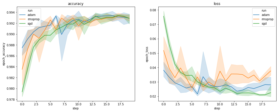
The plots above show the timecourses of validation accuracy and validation loss. Each curve shows the average across 5 runs under an optimizer type. Thanks to a built-in feature of seaborn.lineplot(), each curve also displays ±1 standard deviation around the mean, which gives us a clear sense of the variability in these curves and the significance of the differences among the three optimizer types. This visualization of variability is not yet supported in TensorBoard's GUI.
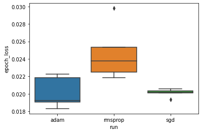
We want to study the hypothesis that the minimum validation loss differs significantly beteen the "adam", "rmsprop" and "sgd" optimizers. So we extract a DataFrame for the minimum validation loss under each of the optimizers.
Then we make a boxplot to visualize the difference in the minimum validation losses.
adam_min_val_loss = dfw_validation.loc[optimizer_validation=="adam", :].groupby(
    "run", as_index=False).agg({"epoch_loss": "min"})
rmsprop_min_val_loss = dfw_validation.loc[optimizer_validation=="rmsprop", :].groupby(
    "run", as_index=False).agg({"epoch_loss": "min"})
sgd_min_val_loss = dfw_validation.loc[optimizer_validation=="sgd", :].groupby(
    "run", as_index=False).agg({"epoch_loss": "min"})
min_val_loss = pd.concat([adam_min_val_loss, rmsprop_min_val_loss, sgd_min_val_loss])

sns.boxplot(data=min_val_loss, y="epoch_loss",
            x=min_val_loss.run.apply(lambda run: run.split(",")[0]))
<matplotlib.axes._subplots.AxesSubplot at 0x7f5e017c8150>

# Perform pairwise comparisons between the minimum validation losses
# from the three optimizers.
_, p_adam_vs_rmsprop = stats.ttest_ind(
    adam_min_val_loss["epoch_loss"],
    rmsprop_min_val_loss["epoch_loss"])
_, p_adam_vs_sgd = stats.ttest_ind(
    adam_min_val_loss["epoch_loss"],
    sgd_min_val_loss["epoch_loss"])
_, p_rmsprop_vs_sgd = stats.ttest_ind(
    rmsprop_min_val_loss["epoch_loss"],
    sgd_min_val_loss["epoch_loss"])
print("adam vs. rmsprop: p = %.4f" % p_adam_vs_rmsprop)
print("adam vs. sgd: p = %.4f" % p_adam_vs_sgd)
print("rmsprop vs. sgd: p = %.4f" % p_rmsprop_vs_sgd)
adam vs. rmsprop: p = 0.0244
adam vs. sgd: p = 0.9749
rmsprop vs. sgd: p = 0.0135
Therefore, at a significance level of 0.05, our analysis confirms our hypothesis that the minimum validation loss is significantly higher (i.e., worse) in the rmsprop optimizer compared to the other two optimizers included in our experiment.
In summary, this tutorial provides an example of how to access scalar data as panda.DataFrames from TensorBoard.dev. It demonstrates the kind of flexible and powerful analyses and visualization you can do with the DataFrames.
