Research tools

TensorFlow Quantum brings quantum primitives into the TensorFlow ecosystem. Now quantum researchers can leverage tools from TensorFlow. In this tutorial you will take a closer look at incorporating TensorBoard into your quantum computing research. Using the DCGAN tutorial from TensorFlow you will quickly build up working experiments and visualizations similar to ones done by Niu et al.. Broadly speaking you will:

Train a GAN to produce samples that look like they came from quantum circuits.
Visualize the training progress as well as distribuion evolution over time.
Benchmark the experiment by exploring the compute graph.

pip install tensorflow==2.15.0 tensorflow-quantum==0.7.3 tensorboard_plugin_profile==2.15.0

# Update package resources to account for version changes.
import importlib, pkg_resources
importlib.reload(pkg_resources)

/tmpfs/tmp/ipykernel_32914/1875984233.py:2: DeprecationWarning: pkg_resources is deprecated as an API. See https://setuptools.pypa.io/en/latest/pkg_resources.html
  import importlib, pkg_resources
<module 'pkg_resources' from '/tmpfs/src/tf_docs_env/lib/python3.9/site-packages/pkg_resources/__init__.py'>

#docs_infra: no_execute
%load_ext tensorboard

import datetime
import time
import cirq
import tensorflow as tf
import tensorflow_quantum as tfq
from tensorflow.keras import layers

# visualization tools
%matplotlib inline
import matplotlib.pyplot as plt
from cirq.contrib.svg import SVGCircuit

2024-12-14 12:47:19.531470: E external/local_xla/xla/stream_executor/cuda/cuda_dnn.cc:9261] Unable to register cuDNN factory: Attempting to register factory for plugin cuDNN when one has already been registered
2024-12-14 12:47:19.531519: E external/local_xla/xla/stream_executor/cuda/cuda_fft.cc:607] Unable to register cuFFT factory: Attempting to register factory for plugin cuFFT when one has already been registered
2024-12-14 12:47:19.533091: E external/local_xla/xla/stream_executor/cuda/cuda_blas.cc:1515] Unable to register cuBLAS factory: Attempting to register factory for plugin cuBLAS when one has already been registered
2024-12-14 12:47:21.540597: E external/local_xla/xla/stream_executor/cuda/cuda_driver.cc:274] failed call to cuInit: CUDA_ERROR_NO_DEVICE: no CUDA-capable device is detected

1. Data generation

Start by gathering some data. You can use TensorFlow Quantum to quickly generate some bitstring samples that will be the primary datasource for the rest of your experiments. Like Niu et al. you will explore how easy it is to emulate sampling from random circuits with drastically reduced depth. First, define some helpers:

def generate_circuit(qubits):
    """Generate a random circuit on qubits."""
    random_circuit = cirq.experiments.random_rotations_between_grid_interaction_layers_circuit(
        qubits, depth=2)
    return random_circuit

def generate_data(circuit, n_samples):
    """Draw n_samples samples from circuit into a tf.Tensor."""
    return tf.squeeze(tfq.layers.Sample()(circuit, repetitions=n_samples).to_tensor())

Now you can inspect the circuit as well as some sample data:

qubits = cirq.GridQubit.rect(1, 5)
random_circuit_m = generate_circuit(qubits) + cirq.measure_each(*qubits)
SVGCircuit(random_circuit_m)

findfont: Font family 'Arial' not found.
findfont: Font family 'Arial' not found.
findfont: Font family 'Arial' not found.
findfont: Font family 'Arial' not found.
findfont: Font family 'Arial' not found.
findfont: Font family 'Arial' not found.
findfont: Font family 'Arial' not found.
findfont: Font family 'Arial' not found.
findfont: Font family 'Arial' not found.
findfont: Font family 'Arial' not found.
findfont: Font family 'Arial' not found.
findfont: Font family 'Arial' not found.
findfont: Font family 'Arial' not found.
findfont: Font family 'Arial' not found.
findfont: Font family 'Arial' not found.
findfont: Font family 'Arial' not found.
findfont: Font family 'Arial' not found.
findfont: Font family 'Arial' not found.
findfont: Font family 'Arial' not found.
findfont: Font family 'Arial' not found.
findfont: Font family 'Arial' not found.
findfont: Font family 'Arial' not found.
findfont: Font family 'Arial' not found.
findfont: Font family 'Arial' not found.
findfont: Font family 'Arial' not found.

svg

samples = cirq.sample(random_circuit_m, repetitions=10)
print('10 Random bitstrings from this circuit:')
print(samples)

10 Random bitstrings from this circuit:
q(0, 0)=0111111001
q(0, 1)=0111101100
q(0, 2)=1101111111
q(0, 3)=1111010011
q(0, 4)=0111111101

You can do the same thing in TensorFlow Quantum with:

generate_data(random_circuit_m, 10)

<tf.Tensor: shape=(10, 5), dtype=int8, numpy=
array([[0, 1, 1, 0, 1],
       [0, 1, 1, 1, 0],
       [1, 0, 1, 0, 0],
       [1, 0, 1, 1, 1],
       [1, 0, 1, 1, 1],
       [1, 0, 1, 1, 1],
       [1, 1, 1, 0, 1],
       [1, 1, 1, 1, 0],
       [1, 1, 1, 1, 1],
       [1, 1, 1, 1, 1]], dtype=int8)>

Now you can quickly generate your training data with:

N_SAMPLES = 60000
N_QUBITS = 10
QUBITS = cirq.GridQubit.rect(1, N_QUBITS)
REFERENCE_CIRCUIT = generate_circuit(QUBITS)
all_data = generate_data(REFERENCE_CIRCUIT, N_SAMPLES)
all_data

<tf.Tensor: shape=(60000, 10), dtype=int8, numpy=
array([[0, 0, 0, ..., 1, 1, 0],
       [0, 0, 0, ..., 1, 1, 1],
       [0, 0, 0, ..., 0, 0, 1],
       ...,
       [1, 1, 1, ..., 1, 1, 1],
       [1, 1, 1, ..., 1, 1, 1],
       [1, 1, 1, ..., 1, 1, 1]], dtype=int8)>

It will be useful to define some helper functions to visualize as training gets underway. Two interesting quantities to use are:

The integer values of samples, so that you can create histograms of the distribution.
The linear XEB fidelity estimate of a set of samples, to give some indication of how "truly quantum random" the samples are.

@tf.function
def bits_to_ints(bits):
    """Convert tensor of bitstrings to tensor of ints."""
    sigs = tf.constant([1 << i for i in range(N_QUBITS)], dtype=tf.int32)
    rounded_bits = tf.clip_by_value(tf.math.round(
        tf.cast(bits, dtype=tf.dtypes.float32)), clip_value_min=0, clip_value_max=1)
    return tf.einsum('jk,k->j', tf.cast(rounded_bits, dtype=tf.dtypes.int32), sigs)

@tf.function
def xeb_fid(bits):
    """Compute linear XEB fidelity of bitstrings."""
    final_probs = tf.squeeze(
        tf.abs(tfq.layers.State()(REFERENCE_CIRCUIT).to_tensor()) ** 2)
    nums = bits_to_ints(bits)
    return (2 ** N_QUBITS) * tf.reduce_mean(tf.gather(final_probs, nums)) - 1.0

Here you can visualize your distribution and sanity check things using XEB:

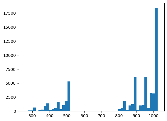
plt.hist(bits_to_ints(all_data).numpy(), 50)
plt.show()

png

xeb_fid(all_data)

WARNING:tensorflow:You are casting an input of type complex64 to an incompatible dtype float32.  This will discard the imaginary part and may not be what you intended.
<tf.Tensor: shape=(), dtype=float32, numpy=0.77480805>

2. Build a model

Here you can use the relevant components from the DCGAN tutorial for the quantum case. Instead of producing MNIST digits the new GAN will be used to produce bitstring samples with length N_QUBITS

LATENT_DIM = 100
def make_generator_model():
    """Construct generator model."""
    model = tf.keras.Sequential()
    model.add(layers.Dense(256, use_bias=False, input_shape=(LATENT_DIM,)))
    model.add(layers.Dense(128, activation='relu'))
    model.add(layers.Dropout(0.3))
    model.add(layers.Dense(64, activation='relu'))
    model.add(layers.Dense(N_QUBITS, activation='relu'))

    return model

def make_discriminator_model():
    """Constrcut discriminator model."""
    model = tf.keras.Sequential()
    model.add(layers.Dense(256, use_bias=False, input_shape=(N_QUBITS,)))
    model.add(layers.Dense(128, activation='relu'))
    model.add(layers.Dropout(0.3))
    model.add(layers.Dense(32, activation='relu'))
    model.add(layers.Dense(1))

    return model

Next, instantiate your generator and discriminator models, define the losses and create the train_step function to use for your main training loop:

discriminator = make_discriminator_model()
generator = make_generator_model()

cross_entropy = tf.keras.losses.BinaryCrossentropy(from_logits=True)
def discriminator_loss(real_output, fake_output):
    """Compute discriminator loss."""
    real_loss = cross_entropy(tf.ones_like(real_output), real_output)
    fake_loss = cross_entropy(tf.zeros_like(fake_output), fake_output)
    total_loss = real_loss + fake_loss
    return total_loss

def generator_loss(fake_output):
    """Compute generator loss."""
    return cross_entropy(tf.ones_like(fake_output), fake_output)

generator_optimizer = tf.keras.optimizers.Adam(1e-4)
discriminator_optimizer = tf.keras.optimizers.Adam(1e-4)

BATCH_SIZE=256

@tf.function
def train_step(images):
    """Run train step on provided image batch."""
    noise = tf.random.normal([BATCH_SIZE, LATENT_DIM])
    with tf.GradientTape() as gen_tape, tf.GradientTape() as disc_tape:
        generated_images = generator(noise, training=True)

        real_output = discriminator(images, training=True)
        fake_output = discriminator(generated_images, training=True)

        gen_loss = generator_loss(fake_output)
        disc_loss = discriminator_loss(real_output, fake_output)

    gradients_of_generator = gen_tape.gradient(
        gen_loss, generator.trainable_variables)
    gradients_of_discriminator = disc_tape.gradient(
        disc_loss, discriminator.trainable_variables)

    generator_optimizer.apply_gradients(
        zip(gradients_of_generator, generator.trainable_variables))
    discriminator_optimizer.apply_gradients(
        zip(gradients_of_discriminator, discriminator.trainable_variables))

    return gen_loss, disc_loss

Now that you have all the building blocks needed for your model, you can setup a training function that incorporates TensorBoard visualization. First setup a TensorBoard filewriter:

logdir = "tb_logs/" + datetime.datetime.now().strftime("%Y%m%d-%H%M%S")
file_writer = tf.summary.create_file_writer(logdir + "/metrics")
file_writer.set_as_default()

Using the tf.summary module, you can now incorporate scalar, histogram (as well as other) logging to TensorBoard inside of the main train function:

def train(dataset, epochs, start_epoch=1):
    """Launch full training run for the given number of epochs."""
    # Log original training distribution.
    tf.summary.histogram('Training Distribution', data=bits_to_ints(dataset), step=0)

    batched_data = tf.data.Dataset.from_tensor_slices(dataset).shuffle(N_SAMPLES).batch(512)
    t = time.time()
    for epoch in range(start_epoch, start_epoch + epochs):
        for i, image_batch in enumerate(batched_data):
            # Log batch-wise loss.
            gl, dl = train_step(image_batch)
            tf.summary.scalar(
                'Generator loss', data=gl, step=epoch * len(batched_data) + i)
            tf.summary.scalar(
                'Discriminator loss', data=dl, step=epoch * len(batched_data) + i)

        # Log full dataset XEB Fidelity and generated distribution.
        generated_samples = generator(tf.random.normal([N_SAMPLES, 100]))
        tf.summary.scalar(
        'Generator XEB Fidelity Estimate', data=xeb_fid(generated_samples), step=epoch)
        tf.summary.histogram(
        'Generator distribution', data=bits_to_ints(generated_samples), step=epoch)
        # Log new samples drawn from this particular random circuit.
        random_new_distribution = generate_data(REFERENCE_CIRCUIT, N_SAMPLES)
        tf.summary.histogram(
        'New round of True samples', data=bits_to_ints(random_new_distribution), step=epoch)

        if epoch % 10 == 0:
            print('Epoch {}, took {}(s)'.format(epoch, time.time() - t))
            t = time.time()

3. Vizualize training and performance

The TensorBoard dashboard can now be launched with:

#docs_infra: no_execute
%tensorboard --logdir tb_logs/

When calling train the TensoBoard dashboard will auto-update with all of the summary statistics given in the training loop.

train(all_data, epochs=50)

Epoch 10, took 9.134180545806885(s)
Epoch 20, took 6.694354772567749(s)
Epoch 30, took 6.628702640533447(s)
Epoch 40, took 6.614518880844116(s)
Epoch 50, took 6.6417601108551025(s)

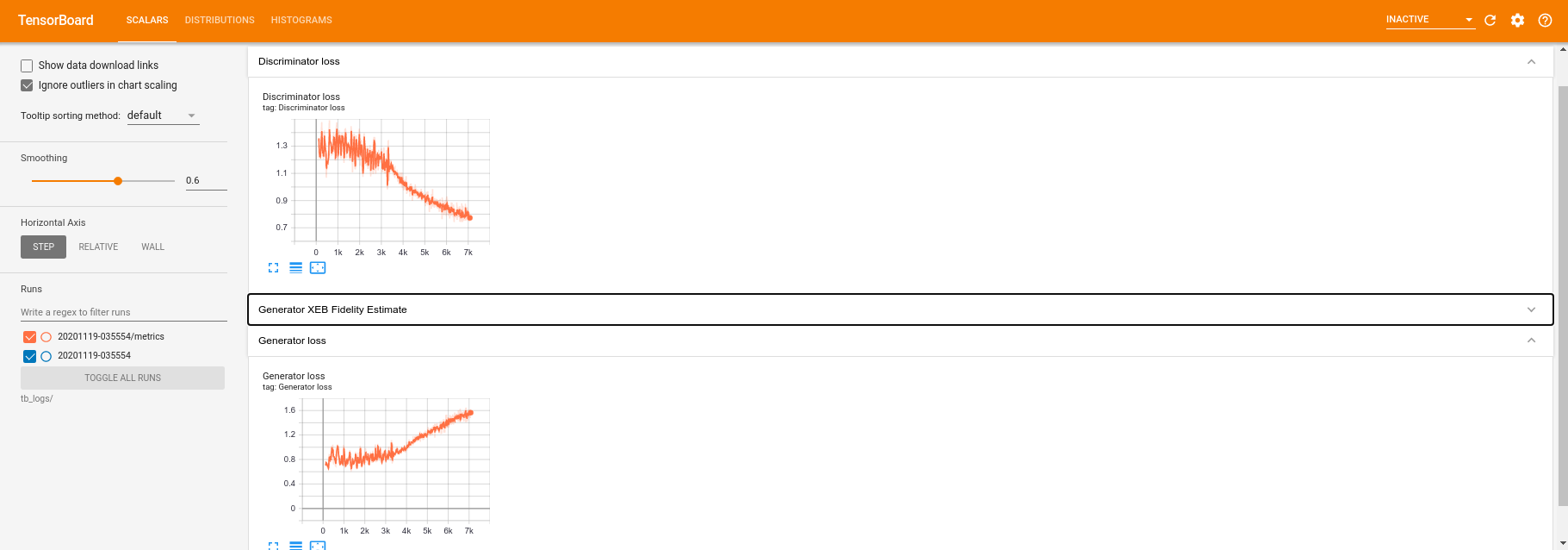
While the training is running (and once it is complete) you can examine the scalar quantities:

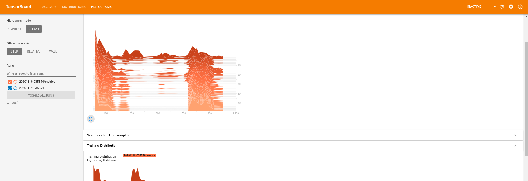
Switching over to the histogram tab you can also see how well the generator network does at recreating samples from the quantum distribution:

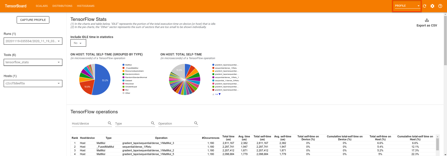
In addition to allowing real time monitoring of summary statistics related to your experiment, TensorBoard can also help you profile your experiments to identify performance bottlenecks. To re-run your model with performance monitoring you can do:

tf.profiler.experimental.start(logdir)
train(all_data, epochs=10, start_epoch=50)
tf.profiler.experimental.stop()

Epoch 50, took 0.7859878540039062(s)

TensorBoard will profile all of the code between tf.profiler.experimental.start and tf.profiler.experimental.stop. This profile data can then be viewed in the profile page of TensorBoard:

Try increasing the depth or experimenting with different classes of quantum circuits. Check out all the other great features of TensorBoard like hyperparameter tuning that you can incorporate into your TensorFlow Quantum experiments.