 View on TensorFlow.org View on TensorFlow.org
|
 Run in Google Colab Run in Google Colab
|
 View source on GitHub View source on GitHub
|
 Download notebook Download notebook
|
In this colab, we explore Gaussian process regression using TensorFlow and TensorFlow Probability. We generate some noisy observations from some known functions and fit GP models to those data. We then sample from the GP posterior and plot the sampled function values over grids in their domains.
Background
Let \(\mathcal{X}\) be any set. A Gaussian process (GP) is a collection of random variables indexed by \(\mathcal{X}\) such that if \(\{X_1, \ldots, X_n\} \subset \mathcal{X}\) is any finite subset, the marginal density \(p(X_1 = x_1, \ldots, X_n = x_n)\) is multivariate Gaussian. Any Gaussian distribution is completely specified by its first and second central moments (mean and covariance), and GP's are no exception. We can specify a GP completely in terms of its mean function \(\mu : \mathcal{X} \to \mathbb{R}\) and covariance function \(k : \mathcal{X} \times \mathcal{X} \to \mathbb{R}\). Most of the expressive power of GP's is encapsulated in the choice of covariance function. For various reasons, the covariance function is also referred to as a kernel function. It is required only to be symmetric and positive-definite (see Ch. 4 of Rasmussen & Williams). Below we make use of the ExponentiatedQuadratic covariance kernel. Its form is
\[ k(x, x') := \sigma^2 \exp \left( \frac{\|x - x'\|^2}{\lambda^2} \right) \]
where \(\sigma^2\) is called the 'amplitude' and \(\lambda\) the length scale. The kernel parameters can be selected via a maximum likelihood optimization procedure.
A full sample from a GP comprises a real-valued function over the entire space \(\mathcal{X}\) and is in practice impractical to realize; often one chooses a set of points at which to observe a sample and draws function values at these points. This is achieved by sampling from an appropriate (finite-dimensional) multi-variate Gaussian.
Note that, according to the above definition, any finite-dimensional multivariate Gaussian distribution is also a Gaussian process. Usually, when one refers to a GP, it is implicit that the index set is some \(\mathbb{R}^n\) and we will indeed make this assumption here.
A common application of Gaussian processes in machine learning is Gaussian process regression. The idea is that we wish to estimate an unknown function given noisy observations \(\{y_1, \ldots, y_N\}\) of the function at a finite number of points \(\{x_1, \ldots x_N\}.\) We imagine a generative process
\[ \begin{align} f \sim \: & \textsf{GaussianProcess}\left( \text{mean_fn}=\mu(x), \text{covariance_fn}=k(x, x')\right) \\ y_i \sim \: & \textsf{Normal}\left( \text{loc}=f(x_i), \text{scale}=\sigma\right), i = 1, \ldots, N \end{align} \]
As noted above, the sampled function is impossible to compute, since we would require its value at an infinite number of points. Instead, one considers a finite sample from a multivariate Gaussian.
\[ \begin{gather} \begin{bmatrix} f(x_1) \\ \vdots \\ f(x_N) \end{bmatrix} \sim \textsf{MultivariateNormal} \left( \: \text{loc}= \begin{bmatrix} \mu(x_1) \\ \vdots \\ \mu(x_N) \end{bmatrix} \:,\: \text{scale}= \begin{bmatrix} k(x_1, x_1) & \cdots & k(x_1, x_N) \\ \vdots & \ddots & \vdots \\ k(x_N, x_1) & \cdots & k(x_N, x_N) \\ \end{bmatrix}^{1/2} \: \right) \end{gather} \\ y_i \sim \textsf{Normal} \left( \text{loc}=f(x_i), \text{scale}=\sigma \right) \]
Note the exponent \(\frac{1}{2}\) on the covariance matrix: this denotes a Cholesky decomposition. Comptuing the Cholesky is necessary because the MVN is a location-scale family distribution. Unfortunately the Cholesky decomposition is computationally expensive, taking \(O(N^3)\) time and \(O(N^2)\) space. Much of the GP literature is focused on dealing with this seemingly innocuous little exponent.
It is common to take the prior mean function to be constant, often zero. Also, some notational conventions are convenient. One often writes \(\mathbf{f}\) for the finite vector of sampled function values. A number of interesting notations are used for the covariance matrix resulting from the application of \(k\) to pairs of inputs. Following (Quiñonero-Candela, 2005), we note that the components of the matrix are covariances of function values at particular input points. Thus we can denote the covariance matrix as \(K_{AB}\) where \(A\) and \(B\) are some indicators of the collection of function values along the given matrix dimensions.
For example, given observed data \((\mathbf{x}, \mathbf{y})\) with implied latent function values \(\mathbf{f}\), we can write
\[ K_{\mathbf{f},\mathbf{f} } = \begin{bmatrix} k(x_1, x_1) & \cdots & k(x_1, x_N) \\ \vdots & \ddots & \vdots \\ k(x_N, x_1) & \cdots & k(x_N, x_N) \\ \end{bmatrix} \]
Similarly, we can mix sets of inputs, as in
\[ K_{\mathbf{f},*} = \begin{bmatrix} k(x_1, x^*_1) & \cdots & k(x_1, x^*_T) \\ \vdots & \ddots & \vdots \\ k(x_N, x^*_1) & \cdots & k(x_N, x^*_T) \\ \end{bmatrix} \]
where we suppose there are \(N\) training inputs, and \(T\) test inputs. The above generative process may then be written compactly as
\[ \begin{align} \mathbf{f} \sim \: & \textsf{MultivariateNormal} \left( \text{loc}=\mathbf{0}, \text{scale}=K_{\mathbf{f},\mathbf{f} }^{1/2} \right) \\ y_i \sim \: & \textsf{Normal} \left( \text{loc}=f_i, \text{scale}=\sigma \right), i = 1, \ldots, N \end{align} \]
The sampling operation in the first line yields a finite set of \(N\) function values from a multivariate Gaussian -- not an entire function as in the above GP draw notation. The second line describes a collection of \(N\) draws from univariate Gaussians centered at the various function values, with fixed observation noise \(\sigma^2\).
With the above generative model in place, we can proceed to consider the posterior inference problem. This yields a posterior distribution over function values at a new set of test points, conditioned on the observed noisy data from the process above.
With the above notation in place, we can compactly write the posterior predictive distribution over future (noisy) observations conditional on corresponding inputs and training data as follows (for more details, see §2.2 of Rasmussen & Williams).
\[ \mathbf{y}^* \mid \mathbf{x}^*, \mathbf{x}, \mathbf{y} \sim \textsf{Normal} \left( \text{loc}=\mathbf{\mu}^*, \text{scale}=(\Sigma^*)^{1/2} \right), \]
where
\[ \mathbf{\mu}^* = K_{*,\mathbf{f} }\left(K_{\mathbf{f},\mathbf{f} } + \sigma^2 I \right)^{-1} \mathbf{y} \]
and
\[ \Sigma^* = K_{*,*} - K_{*,\mathbf{f} } \left(K_{\mathbf{f},\mathbf{f} } + \sigma^2 I \right)^{-1} K_{\mathbf{f},*} \]
Imports
import time

import numpy as np
import matplotlib.pyplot as plt
import tensorflow as tf
import tf_keras
import tensorflow_probability as tfp
tfb = tfp.bijectors
tfd = tfp.distributions
tfk = tfp.math.psd_kernels

from mpl_toolkits.mplot3d import Axes3D
%pylab inline
# Configure plot defaults
plt.rcParams['axes.facecolor'] = 'white'
plt.rcParams['grid.color'] = '#666666'
%config InlineBackend.figure_format = 'png'
Populating the interactive namespace from numpy and matplotlib
Example: Exact GP Regression on Noisy Sinusoidal Data
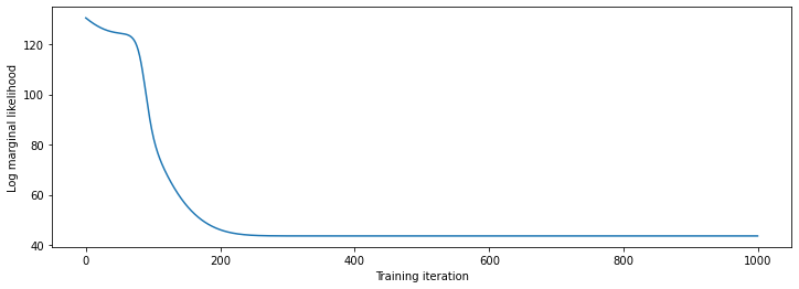
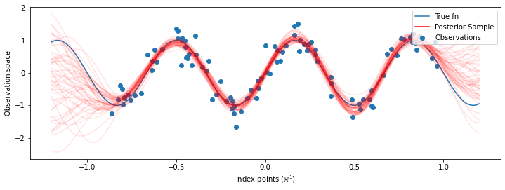
Here we generate training data from a noisy sinusoid, then sample a bunch of curves from the posterior of the GP regression model. We use Adam to optimize the kernel hyperparameters (we minimize the negative log likelihood of the data under the prior). We plot the training curve, followed by the true function and the posterior samples.
def sinusoid(x):
  return np.sin(3 * np.pi * x[..., 0])

def generate_1d_data(num_training_points, observation_noise_variance):
  """Generate noisy sinusoidal observations at a random set of points.

  Returns:
     observation_index_points, observations
  """
  index_points_ = np.random.uniform(-1., 1., (num_training_points, 1))
  index_points_ = index_points_.astype(np.float64)
  # y = f(x) + noise
  observations_ = (sinusoid(index_points_) +
                   np.random.normal(loc=0,
                                    scale=np.sqrt(observation_noise_variance),
                                    size=(num_training_points)))
  return index_points_, observations_
# Generate training data with a known noise level (we'll later try to recover
# this value from the data).
NUM_TRAINING_POINTS = 100
observation_index_points_, observations_ = generate_1d_data(
    num_training_points=NUM_TRAINING_POINTS,
    observation_noise_variance=.1)
We'll put priors on the kernel hyperparameters, and write the joint distribution of the hyperparameters and observed data using tfd.JointDistributionNamed.
def build_gp(amplitude, length_scale, observation_noise_variance):
  """Defines the conditional dist. of GP outputs, given kernel parameters."""

  # Create the covariance kernel, which will be shared between the prior (which we
  # use for maximum likelihood training) and the posterior (which we use for
  # posterior predictive sampling)
  kernel = tfk.ExponentiatedQuadratic(amplitude, length_scale)

  # Create the GP prior distribution, which we will use to train the model
  # parameters.
  return tfd.GaussianProcess(
      kernel=kernel,
      index_points=observation_index_points_,
      observation_noise_variance=observation_noise_variance)

gp_joint_model = tfd.JointDistributionNamed({
    'amplitude': tfd.LogNormal(loc=0., scale=np.float64(1.)),
    'length_scale': tfd.LogNormal(loc=0., scale=np.float64(1.)),
    'observation_noise_variance': tfd.LogNormal(loc=0., scale=np.float64(1.)),
    'observations': build_gp,
})
We can sanity-check our implementation by verifying that we can sample from the prior, and compute the log-density of a sample.
x = gp_joint_model.sample()
lp = gp_joint_model.log_prob(x)

print("sampled {}".format(x))
print("log_prob of sample: {}".format(lp))
sampled {'observation_noise_variance': <tf.Tensor: shape=(), dtype=float64, numpy=2.067952217184325>, 'length_scale': <tf.Tensor: shape=(), dtype=float64, numpy=1.154435715487831>, 'amplitude': <tf.Tensor: shape=(), dtype=float64, numpy=5.383850737703549>, 'observations': <tf.Tensor: shape=(100,), dtype=float64, numpy=
array([-2.37070577, -2.05363838, -0.95152824,  3.73509388, -0.2912646 ,
        0.46112342, -1.98018513, -2.10295857, -1.33589756, -2.23027226,
       -2.25081374, -0.89450835, -2.54196452,  1.46621647,  2.32016193,
        5.82399989,  2.27241034, -0.67523432, -1.89150197, -1.39834474,
       -2.33954116,  0.7785609 , -1.42763627, -0.57389025, -0.18226098,
       -3.45098732,  0.27986652, -3.64532398, -1.28635204, -2.42362875,
        0.01107288, -2.53222176, -2.0886136 , -5.54047694, -2.18389607,
       -1.11665628, -3.07161217, -2.06070336, -0.84464262,  1.29238438,
       -0.64973999, -2.63805504, -3.93317576,  0.65546645,  2.24721181,
       -0.73403676,  5.31628298, -1.2208384 ,  4.77782252, -1.42978168,
       -3.3089274 ,  3.25370494,  3.02117591, -1.54862932, -1.07360811,
        1.2004856 , -4.3017773 , -4.95787789, -1.95245901, -2.15960839,
       -3.78592731, -1.74096185,  3.54891595,  0.56294143,  1.15288455,
       -0.77323696,  2.34430694, -1.05302007, -0.7514684 , -0.98321063,
       -3.01300144, -3.00033274,  0.44200837,  0.45060886, -1.84497318,
       -1.89616746, -2.15647664, -2.65672581, -3.65493379,  1.70923375,
       -3.88695218, -0.05151283,  4.51906677, -2.28117003,  3.03032793,
       -1.47713194, -0.35625273,  3.73501587, -2.09328047, -0.60665614,
       -0.78177188, -0.67298545,  2.97436033, -0.29407932,  2.98482427,
       -1.54951178,  2.79206821,  4.2225733 ,  2.56265198,  2.80373284])>}
log_prob of sample: -194.96442183797524
Now let's optimize to find the parameter values with highest posterior probability. We'll define a variable for each parameter, and constrain their values to be positive.
# Create the trainable model parameters, which we'll subsequently optimize.
# Note that we constrain them to be strictly positive.

constrain_positive = tfb.Shift(np.finfo(np.float64).tiny)(tfb.Exp())

amplitude_var = tfp.util.TransformedVariable(
    initial_value=1.,
    bijector=constrain_positive,
    name='amplitude',
    dtype=np.float64)

length_scale_var = tfp.util.TransformedVariable(
    initial_value=1.,
    bijector=constrain_positive,
    name='length_scale',
    dtype=np.float64)

observation_noise_variance_var = tfp.util.TransformedVariable(
    initial_value=1.,
    bijector=constrain_positive,
    name='observation_noise_variance_var',
    dtype=np.float64)

trainable_variables = [v.trainable_variables[0] for v in
                       [amplitude_var,
                       length_scale_var,
                       observation_noise_variance_var]]
To condition the model on our observed data, we'll define a target_log_prob function, which takes the (still to be inferred) kernel hyperparameters.
def target_log_prob(amplitude, length_scale, observation_noise_variance):
  return gp_joint_model.log_prob({
      'amplitude': amplitude,
      'length_scale': length_scale,
      'observation_noise_variance': observation_noise_variance,
      'observations': observations_
  })
# Now we optimize the model parameters.
num_iters = 1000
optimizer = tf_keras.optimizers.Adam(learning_rate=.01)

# Use `tf.function` to trace the loss for more efficient evaluation.
@tf.function(autograph=False, jit_compile=False)
def train_model():
  with tf.GradientTape() as tape:
    loss = -target_log_prob(amplitude_var, length_scale_var,
                            observation_noise_variance_var)
  grads = tape.gradient(loss, trainable_variables)
  optimizer.apply_gradients(zip(grads, trainable_variables))
  return loss

# Store the likelihood values during training, so we can plot the progress
lls_ = np.zeros(num_iters, np.float64)
for i in range(num_iters):
  loss = train_model()
  lls_[i] = loss

print('Trained parameters:')
print('amplitude: {}'.format(amplitude_var._value().numpy()))
print('length_scale: {}'.format(length_scale_var._value().numpy()))
print('observation_noise_variance: {}'.format(observation_noise_variance_var._value().numpy()))
Trained parameters:
amplitude: 0.9176153445125278
length_scale: 0.18444082442910079
observation_noise_variance: 0.0880273312850989
# Plot the loss evolution
plt.figure(figsize=(12, 4))
plt.plot(lls_)
plt.xlabel("Training iteration")
plt.ylabel("Log marginal likelihood")
plt.show()

# Having trained the model, we'd like to sample from the posterior conditioned
# on observations. We'd like the samples to be at points other than the training
# inputs.
predictive_index_points_ = np.linspace(-1.2, 1.2, 200, dtype=np.float64)
# Reshape to [200, 1] -- 1 is the dimensionality of the feature space.
predictive_index_points_ = predictive_index_points_[..., np.newaxis]

optimized_kernel = tfk.ExponentiatedQuadratic(amplitude_var, length_scale_var)
gprm = tfd.GaussianProcessRegressionModel(
    kernel=optimized_kernel,
    index_points=predictive_index_points_,
    observation_index_points=observation_index_points_,
    observations=observations_,
    observation_noise_variance=observation_noise_variance_var,
    predictive_noise_variance=0.)

# Create op to draw  50 independent samples, each of which is a *joint* draw
# from the posterior at the predictive_index_points_. Since we have 200 input
# locations as defined above, this posterior distribution over corresponding
# function values is a 200-dimensional multivariate Gaussian distribution!
num_samples = 50
samples = gprm.sample(num_samples)
# Plot the true function, observations, and posterior samples.
plt.figure(figsize=(12, 4))
plt.plot(predictive_index_points_, sinusoid(predictive_index_points_),
         label='True fn')
plt.scatter(observation_index_points_[:, 0], observations_,
            label='Observations')
for i in range(num_samples):
  plt.plot(predictive_index_points_, samples[i, :], c='r', alpha=.1,
           label='Posterior Sample' if i == 0 else None)
leg = plt.legend(loc='upper right')
for lh in leg.legendHandles:
    lh.set_alpha(1)
plt.xlabel(r"Index points ($\mathbb{R}^1$)")
plt.ylabel("Observation space")
plt.show()

Marginalizing hyperparameters with HMC
Instead of optimizing the hyperparameters, let's try integrating them out with Hamiltonian Monte Carlo. We'll first define and run a sampler to approximately draw from the posterior distribution over kernel hyperparameters, given the observations.
num_results = 100
num_burnin_steps = 50

sampler = tfp.mcmc.TransformedTransitionKernel(
    tfp.mcmc.NoUTurnSampler(
        target_log_prob_fn=target_log_prob,
        step_size=tf.cast(0.1, tf.float64)),
    bijector=[constrain_positive, constrain_positive, constrain_positive])

adaptive_sampler = tfp.mcmc.DualAveragingStepSizeAdaptation(
    inner_kernel=sampler,
    num_adaptation_steps=int(0.8 * num_burnin_steps),
    target_accept_prob=tf.cast(0.75, tf.float64))

initial_state = [tf.cast(x, tf.float64) for x in [1., 1., 1.]]
# Speed up sampling by tracing with `tf.function`.
@tf.function(autograph=False, jit_compile=False)
def do_sampling():
  return tfp.mcmc.sample_chain(
      kernel=adaptive_sampler,
      current_state=initial_state,
      num_results=num_results,
      num_burnin_steps=num_burnin_steps,
      trace_fn=lambda current_state, kernel_results: kernel_results)

t0 = time.time()
samples, kernel_results = do_sampling()
t1 = time.time()
print("Inference ran in {:.2f}s.".format(t1-t0))
Inference ran in 9.00s.
Let's sanity-check the sampler by examining the hyperparameter traces.
(amplitude_samples,
 length_scale_samples,
 observation_noise_variance_samples) = samples

f = plt.figure(figsize=[15, 3])
for i, s in enumerate(samples):
  ax = f.add_subplot(1, len(samples) + 1, i + 1)
  ax.plot(s)

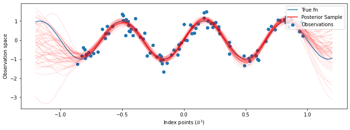
Now instead of constructing a single GP with the optimized hyperparameters, we construct the posterior predictive distribution as a mixture of GPs, each defined by a sample from the posterior distribution over hyperparameters. This approximately integrates over the posterior parameters via Monte Carlo sampling to compute the marginal predictive distribution at unobserved locations.
# The sampled hyperparams have a leading batch dimension, `[num_results, ...]`,
# so they construct a *batch* of kernels.
batch_of_posterior_kernels = tfk.ExponentiatedQuadratic(
    amplitude_samples, length_scale_samples)

# The batch of kernels creates a batch of GP predictive models, one for each
# posterior sample.
batch_gprm = tfd.GaussianProcessRegressionModel(
    kernel=batch_of_posterior_kernels,
    index_points=predictive_index_points_,
    observation_index_points=observation_index_points_,
    observations=observations_,
    observation_noise_variance=observation_noise_variance_samples,
    predictive_noise_variance=0.)

# To construct the marginal predictive distribution, we average with uniform
# weight over the posterior samples.
predictive_gprm = tfd.MixtureSameFamily(
    mixture_distribution=tfd.Categorical(logits=tf.zeros([num_results])),
    components_distribution=batch_gprm)

num_samples = 50
samples = predictive_gprm.sample(num_samples)
# Plot the true function, observations, and posterior samples.
plt.figure(figsize=(12, 4))
plt.plot(predictive_index_points_, sinusoid(predictive_index_points_),
         label='True fn')
plt.scatter(observation_index_points_[:, 0], observations_,
            label='Observations')
for i in range(num_samples):
  plt.plot(predictive_index_points_, samples[i, :], c='r', alpha=.1,
           label='Posterior Sample' if i == 0 else None)
leg = plt.legend(loc='upper right')
for lh in leg.legendHandles:
    lh.set_alpha(1)
plt.xlabel(r"Index points ($\mathbb{R}^1$)")
plt.ylabel("Observation space")
plt.show()

Although the differences are subtle in this case, in general, we would expect the posterior predictive distribution to generalize better (give higher likelihood to held-out data) than just using the most likely parameters as we did above.
